Going from Primus to Primus V3

PrimusWhere we started

The year is 2025. Computer Vision is entirely occupied by the transformers. Well, not entirely... One small sub-field of Computer Vision still holds out against the invaders...

Vision transformers took over natural images years ago, but in 3D medical image analysis CNNs still dominated the benchmarks. The reasons why were unclear at the time. Maybe it was because datasets in our domain are usually only in the hundreds of cases instead of tens of thousands or millions. Maybe it was because volumes are so large that we had to work with 3D image crops. These result in shorter distances within an image, which might make the smaller receptive field of the CNNs less problematic. Maybe it was due to the tokenisation of 3D volumes being very coarse to keep the sequence length short. There were many reasons that could explain this.

Initially, we took apart nine popular transformer-based networks for medical image segmentation (Lost in Transformation). Most of them hide a substantial CNN inside. When we replaced their transformer blocks with identity mappings, many still retained almost all of their performance. In these architectures the convolutions were able to compensate for the absence of the transformer blocks. This showed that the transformers were not needed to reach high performance, calling their contribution into question.

Primus was our initial attempt to build the opposite: an architecture where the transformer has to do the work. We started from the plain vision transformer recipe and kept almost all parameters and FLOPs inside the transformer. The input crop is tokenized with a patch size of 8×8×8 voxels (instead of the usual 16×16×16) by a single strided conv, the tokens pass through a transformer with 3D rotary position embeddings, SwiGLU, LayerScale and DropPath, and a lightweight decoder turns them back into a segmentation. Learning rate and weight decay were tuned to static values that work well across datasets. Everything else, from preprocessing to augmentation recipes, was taken as-is from nnU-Net.

This recipe worked, up to a point. Primus reached parity with the best hybrid architecture and left most of the others behind, while relying mostly on attention. When we removed its transformer blocks, the average Dice score dropped from 88 to 20. But the strong CNNs were still clearly ahead.

So what was missing? The usual argument for transformers is that attention connects every token to every other token and captures long-range dependencies that convolutions cannot. If that were what 3D segmentation needs, Primus should have done better. We had two suspicions: the long-range context doesn't matter much, and the thing that does matter was being lost in the tokenizer.

Problem 1How much context does 3D segmentation need?

In the same analysis paper we tested whether the long-range argument holds. We took a 3D nnU-Net on AMOS (abdominal CT, resampled to 2 × 0.71 × 0.71 mm) and removed resolution stages from the bottom of the U. Every stage we remove shrinks the receptive field, the region of the input that can influence one output voxel. At full depth, the receptive field is limited by the crop itself: 64 × 160 × 192 voxels, or about 13 × 11 × 14 cm, which already covers only part of the abdomen.

With four stages, each output voxel has a receptive field of 32 × 68 × 68 voxels, about 6.4 × 4.8 × 4.8 cm or 7.5% of the input image, and the network still reaches 87.13 Dice against 88.94 at full depth. Dice only drops sharply once the window shrinks to 14 × 32 × 32 voxels, under 3 cm across. This indicates that, for organs in abdominal CT, the label of a voxel is mostly decided by its local neighbourhood. Global context adds a little on top, but it is not where most of the Dice comes from.

Less context, more Dice

We observed a second piece of evidence for this in a Primus ablation experiment. In the Primus paper we halved the crop size along every axis, so the transformer sees one eighth of the volume, and in a second step also shrank the tokens from 8×8×8 to 4×4×4. The 4³ model on the half crop size has exactly as many tokens as the 8³ model on the full crop size, so the transformer's sequence length stays the same; it just works on smaller tokens and less global context.

The key observation we had was that for some datasets halving the crop size while keeping the patch size constant improved performance! Specifically, ACDC and SBM improved in performance for most of the evaluated architectures (including CNNs). This was very unexpected for us at the time, as we had assumed more context would usually help (nnU-Net's preferred scaling axis with growing VRAM availability is usually crop size.) There were of course examples where this field-of-view limitation hurt, such as AMOS, where the performance dropped for all architectures.

To us this clearly indicated that more global context is not always better. At least not for all 3D medical image segmentation tasks.

Problem 2Small structures and the 8×8×8 token

A second insight from the ablation experiment in Table 1 was that the 8×8×8 tokens were sometimes insufficient for small structures. Primus V1 turns every 8×8×8 block of voxels into one token with a single linear projection, a convolution whose kernel and stride are both 8. For large organs this was fine. However, for small structures like those in the Stanford Brain Metastases dataset (SBM) it was not. Primus-M reached 57.63 Dice with 8×8×8 patches, compared with 66.52 for the default nnU-Net. Brain metastases are often smaller than 0.05 cm³. At 1 mm isotropic spacing, that is about a tenth of all voxels in a token.

My working hypothesis for this was a counting argument. Picture a lesion as a small blip of intensity that can be caught by a 3×3×3 conv kernel. Inside one 8×8×8 token that pattern can sit at 6 × 6 × 6 = 216 different offsets. A linear patch embedding has no weight sharing inside the token, so to respond to the blip wherever it sits, it needs a separate weight template for every offset: 216 output dimensions for one tiny pattern. Primus-S only has 396 in total. If one used a single 3×3×3 conv it could learns the same detector once, with 27 weights. This problem also largely disappears when we use 4×4×4 tokens, as the possible space of offsets is much smaller (2 × 2 × 2 = 8). This is also our hypothesis for why Primus V1 with 4×4×4 tokens is so much better on SBM.

Of course, one could circumvent this by making the projection lossless, i.e. flattening the raw 512 voxel intensities of a token into a 512-dimensional embedding and letting the transformer figure it all out. This clearly does not solve the problem. It just hopes that the transformer will fix our laziness and it would also be impossible for small embedding dimensions, such as Primus-S with 396-dimensional tokens. We tried to find elegant solutions for this, but, in the end, we decided to re-introduce the CNN inductive biases into the architecture, as they fit the problem so well.

Primus → V2Put the convolution back into the tokenizer

Primus V2 replaces the single 8×8×8 projection with a small convolutional encoder that follows the downsampling pattern of a U-Net: a 3×3×3 stem at full resolution, then three stride-2 stages that bring the resolution down to 1/8, and a 1×1×1 projection to the embedding dimension. Each resolution gets only one residual block, because we want to minimize weights in the tokenizer. The whole tokenizer of Primus V2-S has about one million parameters.

Before committing to a particular tokenizer, we evaluated different variants, each trained with and without the transformer. Across all tokenizers we evaluated, we found that convolutional tokenizers beat the linear projection, and overlapping 3×3×3 kernels with residual blocks work best among the minimal designs (88.91 Dice versus 88.63 for non-overlapping 2×2×2 projections; plain 3×3×3 convolutions without residuals tie at 88.62). And the stronger the tokenizer, the less the network needs its transformer: with a large residual tokenizer, removing the transformer costs only 1.6 Dice. While the large residual tokenizer might be best overall, we believed using it would defeat the point of Primus, so Primus V2 uses the minimal residual tokenizer, where removing the transformer still costs about 5 Dice.

With this tokenizer, the brain metastases performance gap closes. Primus V2-M reaches 66.36 Dice on SBM, up from 57.63, on par with the default nnU-Net, which performed better than ResEnc-L on this dataset. Averaged over all nine datasets, Primus V2-M lands at 81.43, within 0.05 Dice of ResEnc-L. Primus V2 also represents the latest architecture version of Primus that made it into our TMLR paper.

Problem 3A bottleneck hiding in the tokenizer

After Primus V2 was accepted, Luc Bouteille, a student at IKIM (University Hospital Essen), pointed out something we had missed. The Primus V2 tokenizer grows its channels even more slowly than an nnU-Net encoder does. nnU-Net doubles its encoder channels every time the resolution halves, up to a cap of 320. The Primus V2 tokenizer has 32 channels in the stem and keeps those 32 after the first downsampling stage, then goes to 64 and 128 after the other two. Over the same path, the spatial extent of the input shrinks from 8×8×8 voxels to a single token, a compression factor of 512.

Let's take a look how many values are compressed into a token throughout the tokenizer: In the stem it is 32 channels × 512 voxels = 16,384 values. After three downsampling stages it is 32 × 64 = 2,048, then 64 × 8 = 512 and finally 128 × 1 = 128. The final 1×1×1 projection is linear, so every token embedding is an affine function of those 128 numbers. Whatever the embedding dimension (396 for Primus-S, 864 for Primus-M, 1,056 for Primus-L), the image content that enters the transformer lives in a subspace of at most 128 dimensions. For Primus-M, that is less than a sixth of the transformers embedding dimension.

Doubling channels per halving of resolution is the standard CNN recipe, and even that loses a factor of four per stage here, because each halving divides the number of voxels by eight. For nnU-Net this is not problematic, because the skip connections from the encoder keep the information intact for the decoder. However, in the case of Primus V2, there are no skips and the channel growth is not large enough to avoid an early bottleneck. So the compression limits what reaches the transformer and what can be learned overall.

V2 → V3Wider channels and skip tokens

We tried two ways to remove the bottleneck.

Grow the channels faster

The simplest fix keeps the Primus V2 structure and changes the channel schedule, growing by 2×, 4× and 4× per stage instead of V2's 1×, 2× and 2×, which gives 32 → 64 → 256 → 1,024. We tried several schedules and settled on this one; it is the one used in all experiments below. At 1,024 channels the last level is wider than the token for Primus-S, -B and -M and only slightly narrower than the 1,056 of Primus-L, so the ceiling effectively disappears. The price is a much heavier tokenizer, since the 3×3×3 convolutions at 256 and 1,024 channels are expensive.

Skip connections into the tokens

Luc's proposal tries to solve the problem differently. Instead of forcing everything through the last stage, every intermediate resolution is projected directly onto the token grid and all of these are joined through addition. The stem output is projected through an 8×8×8 convolution with stride 8, the ↓2 output through 4×4×4 with stride 4, and the ↓4 output through 2×2×2 with stride 2. The stem branch is essentially the Primus V1 tokenizer applied to 32 learned channels instead of raw intensities. Each token becomes the sum of all these tokenization schemes at once. The skip branches are scaled by learnable factors initialised at 10⁻⁵, so training starts from the plain tokenizer and leverages the shortcuts as needed.

Primus V3 uses both: the 32 → 64 → 256 → 1,024 schedule and the skip projections. You can compare it with the other tokenizers in Figure 5.

Results on the development datasets

We ran the ablations at the S scale with five folds on our four development datasets (ACDC, AMOS22, KiTS23, LiTS), adding one change at a time on top of Primus V2-S: first the 32 → 64 → 256 → 1,024 channel schedule on its own, then the skip tokens on top of it, which gives Primus V3-S.

Both changes help, and synergize. The wider channels alone lift the development average from 87.68 to 88.00 Dice, level with ResEnc-L (87.97), and beat Primus V2-S. The skip tokens bring Primus V3-S to 88.17 and beat the version without skips in 16 of 20 evaluated dataset-fold pairs. Compared with Primus V2-S, Primus V3-S is better in 18 of 20 dataset-fold pairs and on every dataset. The absolute differences are small, as they tend to be once a method is close to the CNN baselines on these datasets, but they were consistent in our experiments.

Results on all nine datasets

We evaluated Primus V3-S on all nine datasets of the original paper. Primus V3-S improved on Primus V2-S on eight of the nine datasets, with the largest gains observed on MAMA-MIA, ATLAS22 and WORD (+1.0 to +1.1 Dice each), and raised the nine-dataset average from 81.23 to 81.70. The exception is SBM, the dataset that motivated Primus V2, where Primus V3-S lost 2.3 Dice and ends up even with ResEnc-L instead of ahead of it. This was a bit confusing to us, as the tokenizer should be more powerful now, allowing for easier recognition of metastases. However, performance was still not as horrible as it used to be with Primus V1, so we decided to accept this result and leave it at that.

Primus → V2 → V3Where Primus stands now

Primus V3-S reaches 81.70 Dice on average, level with MedNeXt-L (81.72) and slightly ahead of ResEnc-L (81.48). It does so with 70.6M parameters, fewer than ResEnc-L (102.4M) and less than half of Primus V2-M (147.2M). Overall it performs well across all datasets, sometimes yielding the highest scores, and sometimes being close to the best.

Getting from Primus to Primus V3 took us quite a while. In the end, we were able to push Primus V3 to be on par with MedNeXt-L, which was nice for us. However, we also tried many other things that did not work, and we want to share those with you as well in case you find them interesting.

Dead endsWhat we tried that didn't work

Muon for the transformer weights

Muon has been used in NLP for a while. We were wondering whether it could accelerate our transformer training as well. We tried optimizing the transformer's weights with the Muon optimizer and kept AdamW for the convolutional weights. Unfortunately, it did not beat our pure AdamW optimizer setup, so every Primus model is still trained with AdamW.

A heavier decoder

Primus decodes its tokens with a deliberately light stack of transposed convolutions. We tried larger custom decoders of three sizes. None of them helped. The small one gained a bit (but not significantly), the base one lost a bit, and the large one diverged on ATLAS at our default learning rate. Lowering the learning rate tenfold fixed the stability but not the performance.

GoldenGate RoPE

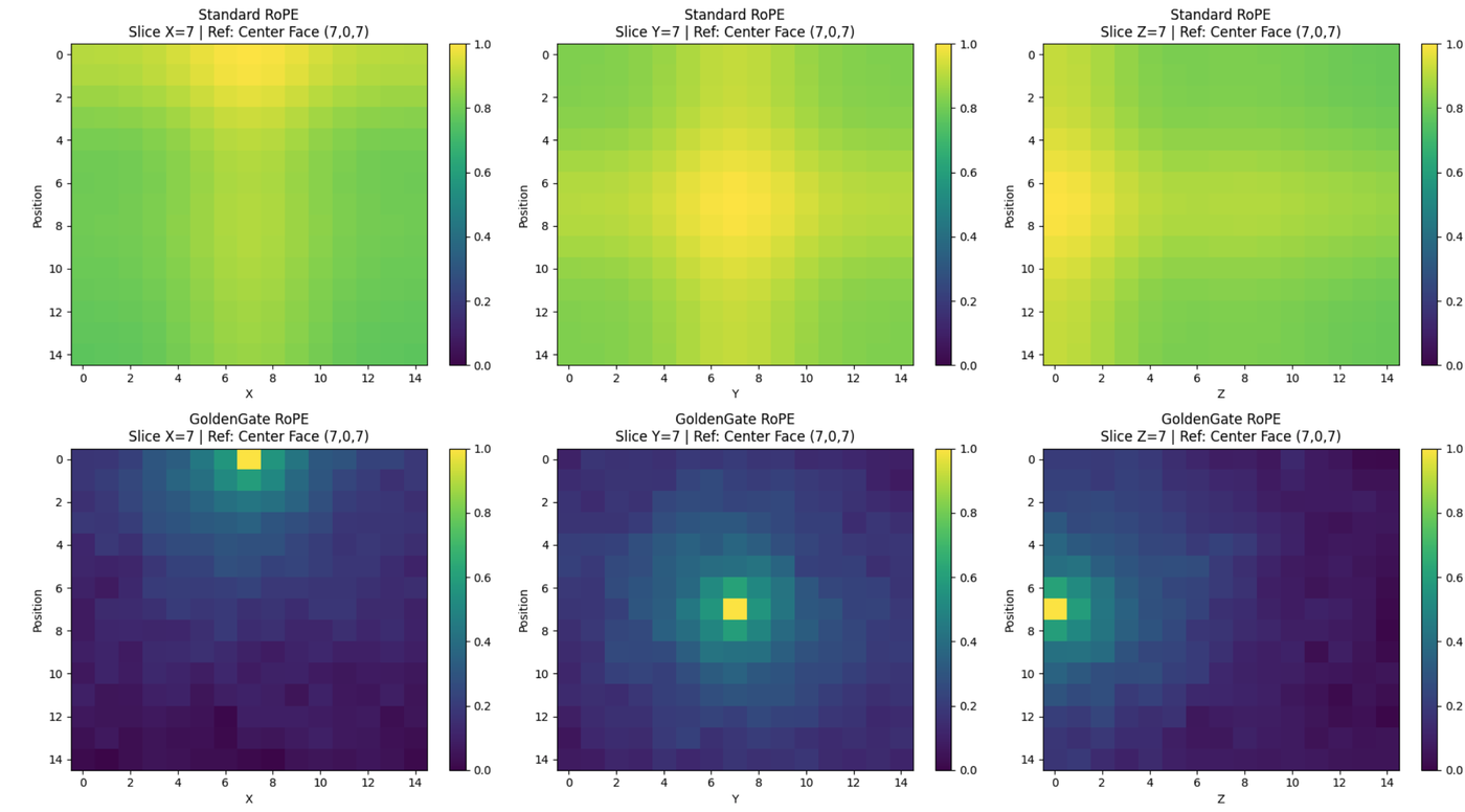
The default RoPE implementation in Primus is a 3D axial RoPE. Axial RoPE leads to high similarity between tokens that are far apart in 3D space but happen to share one or two coordinates. We were not sure if this is a problem, but we expected there to be some benefit to having a more "round" RoPE, where similarity is a function of the Euclidean distance between tokens. GoldenGate RoPE achieves this by spreading the rotation frequencies over many directions chosen with the golden ratio, instead of splitting them across the three axes as axial RoPE does. We swept different minimum and maximum frequencies on the four development datasets. Thirteen of the 28 settings collapsed to near-zero Dice on at least one dataset. Of the 7 settings that finished all four datasets without collapsing, the best reached 86.93, 1.2 below the axial-RoPE reference in the same sweep (88.11).

Positional similarity to one reference tokenSimilarity of the RoPE embedding at every position of a 15×15×15 token grid to the reference at (7, 0, 7). Top: standard axial RoPE. Bottom: GoldenGate RoPE.

Windowing before the convolutions

Overlapping convolutions mean that neighbouring tokens share input voxels, which causes trouble for masked pre-training (see below). So we tried cutting the volume into 8×8×8 windows first and running the tokenizer's convolutions inside each window, so that every token only ever sees its own voxels. These tokenizers did not perform as well as the minimal residual tokenizer, but were still better than Primus V1. We hypothesize that this might be due to boundary artifacts. In an 8×8×8 window, only 6³ = 216 of the 512 voxels have a complete 3×3×3 neighbourhood. The other 58% sit at the window border and see truncated context, and the initial convolutions lose the cross-boundary information that might be important for small targets.

Open problemsCurrent limitations

Masked pre-training with overlapping tokens

Masked image modelling is harder with Primus V2 and V3. With the V1 tokenizer, masking a token hides exactly its 8×8×8 voxels. With overlapping 3×3×3 convolutions, a token's features also depend on voxels of its neighbours, so a visible token next to a masked one ends up partially masked. The network sees such half-masked tokens during pre-training but never at test time, which is a domain shift. SparK-style re-masking of the convolution outputs keeps the mask consistent through the tokenizer, and keeping the normalization layers from seeing masked positions helps further. Pre-training with masking remains harder than with the plain Primus tokenizer.

Only evaluated on segmentation

Our entire evaluation pipeline is based on segmentation. Back when we started this project, there were hardly any large MR or CT classification or report generation datasets available. We would have liked to include some experiments with our architecture on these tasks, but the lack of a classification framework made this non-trivial to do. Lastly, our initial experiments about the importance of global information would most likely yield very different results on the newer classification or report generation tasks. E.g., detecting cardiomegaly is usually about relating heart size to chest size, a task that clearly requires global context. So our earlier insights about the importance of global context do not hold for all tasks.

Long Sequence lengths

Currently, all Primus versions tokenize voxel cubes of 8×8×8 voxels into a single token. While this is a good trade-off for segmentation, this compression leads to a lot of tokens for large 3D volumes. E.g., in COLIPRI, where we used Primus V1, we ablated training with crop-sizes between 128³ and 224³. This leads to sequence lengths between 4.096 and 21.952, which can cost a lot of VRAM and slow down training time. If one were to find a better way of tokenizing the input into larger patches, this could play in ones favor as it also cubically reduces the sequence length. Alternatively, interesting directions to address this are token merging/dropping techniques (since a lot of tokens are probably very redundant) or using sub-quadratic attention mechanisms. Unfortunately, both of these directions are non-trivial hence we leave them for future work.

TakeawaysWhat we learned

• Global context matters less than expected for dense 3D segmentation. On AMOS, a receptive field covering a few percent of the crop already gets most of the way, and at a fixed token budget, smaller patches beat a larger crop. Architectures should be judged on how well they keep local detail.
• Inductive biases belong in the tokenizer. A transformer on top of convolutional tokens is competitive with the best CNNs; the same transformer on top of linear patches is not.
• Make sure you don't hamstring yourself. If channels grow more slowly than resolution shrinks, part of the embedding dimension is decorative. Counting the numbers per token footprint at each level takes a minute and would have caught this earlier.
• Outside eyes help. The bottleneck that Primus V3 fixes was spotted by a student reading our code.

CodeTry it

All three versions are available as trainers in nnU-Net, and we currently recommend Primus V3-S. The crop size (nnU-Net's patch_size) needs to be divisible by 8.

nnUNetv2_train DATASET_ID 3d_fullres FOLD -tr nnUNet_PrimusV3S_Trainer

# earlier versions
nnUNet_Primus_{S,B,M,L}_Trainer     # Primus (linear 8³ tokens)
nnUNet_PrimusV2{S,B,M,L}_Trainer    # PrimusV2 (TMLR version)
nnUNet_PrimusV3{S,B,M,L}_Trainer    # PrimusV3

The architectures themselves live in dynamic-network-architectures. Thanks to Luc Bouteille for the skip-token idea and the careful look at our tokenizer, and to my co-authors Saikat Roy, Fabian Isensee, Constantin Ulrich, Sebastian Ziegler, Dasha Trofimova, Raphael Stock, Michael Baumgartner and Klaus Maier-Hein.

ReferencesFurther reading

1. T. Wald*, S. Roy*, F. Isensee*, et al. Primus: Enforcing Attention Usage for 3D Medical Image Segmentation. TMLR, 2026. arXiv:2503.01835.
2. Lost in Transformation: Current Roadblocks for Transformers in 3D Medical Image Segmentation. OpenReview, 2024.
3. Primus in nnU-Net: documentation, trainers and the PrimusV3 notes.
4. J. Xiong. On N-dimensional Rotary Positional Embeddings (GoldenGate RoPE). 2025.
5. K. Tian et al. Designing BERT for Convolutional Networks: Sparse and Hierarchical Masked Modeling (SparK). ICLR, 2023.

@article{wald2026primus,
  title   = {Primus: Enforcing Attention Usage for 3D Medical Image Segmentation},
  author  = {Wald, Tassilo and Roy, Saikat and Isensee, Fabian and Ulrich, Constantin and
             Ziegler, Sebastian and Trofimova, Dasha and Stock, Raphael and
             Baumgartner, Michael and Maier-Hein, Klaus},
  journal = {Transactions on Machine Learning Research},
  year    = {2026},
  url     = {https://openreview.net/forum?id=x4vZE4PDEu}
}

Written by Tassilo Wald. Questions or corrections: tassilo.wald (at) gmail.com · Back to the homepage